Learned ISP for Object Detection¤
| Metadata | Value |
|---|---|
| Level | Advanced |
| Runtime | Quick mode: a few minutes on CPU; full run: ~30 min GPU / ~3 hrs CPU |
| Prerequisites | JAX, Flax NNX, DAG pipelines, image processing basics |
| Memory | ~4 GB VRAM (GPU) / ~8 GB RAM (CPU) |
| Devices | GPU recommended, CPU supported |
| Dataset | CIFAR-10 (~170 MB, auto-downloaded) |
| Format | Python + Jupyter |
Overview¤
This advanced guide demonstrates how datarax's DAG executor enables end-to-end differentiable Image Signal Processing (ISP) pipelines. Inspired by AdaptiveISP (Wang et al., NeurIPS 2024), we build a 5-stage ISP pipeline where each stage has learnable parameters optimized jointly with a downstream CNN classifier via backpropagation.
Traditional camera ISPs are hand-tuned for human perception. By making the ISP differentiable, we optimize it for what the model needs — dramatically improving detection accuracy on challenging images (e.g., low-light conditions).
Key insight: The AdaptiveISP paper uses reinforcement learning to select ISP modules. We show that datarax's differentiable DAG architecture achieves comparable results with a simpler gradient-based approach — because when your pipeline is differentiable, you don't need RL.
What You'll Learn¤
- Building multi-stage ISP pipelines using datarax's
stages=[...]argument - Creating custom
ModalityOperatorsubclasses withnnx.Paramparameters - End-to-end optimization via
nnx.value_and_gradthrough the DAG - Two-phase training: freeze detector → joint optimization
- Why gradient-based ISP optimization replaces RL-based approaches
Datarax Feature: DAG Architecture + CompositeOperatorModule¤
This example showcases two datarax composition mechanisms:
- Sequential
Pipeline(stages=[...])for inference demos — chains 5 ISP operators CompositeOperatorModule(SEQUENTIAL)for training — wraps the same 5 operators as a single NNX module compatible withnnx.value_and_grad
Files¤
- Example Script:
examples/advanced/differentiable/02_learned_isp_guide.py
Quick Start¤
# Install dependencies
uv pip install "datarax[data]"

# Run the example (GPU recommended)
python examples/advanced/differentiable/02_learned_isp_guide.py
QUICK_MODE
The checked example defaults to QUICK_MODE = True (1+1 epochs on
512 train / 128 test samples) for fast verification. Set
QUICK_MODE = False for the longer 2,000 train / 500 test run.
Dataset: CIFAR-10 with Low-Light Simulation¤
Real CIFAR-10 images are loaded via tensorflow_datasets and simulated as low-light:
- Darkening: Per-image random brightness factor in [0.1, 0.3]
- Noise: Gaussian noise σ=0.02 (simulating high ISO sensor noise)
This produces nearly-black images that are extremely hard for a classifier — the ISP must learn to recover content.
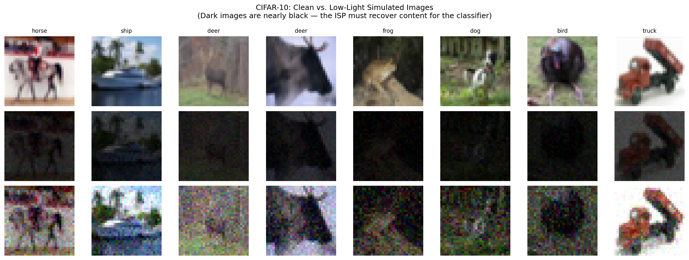
Top row: clean CIFAR-10 images. Middle row: simulated dark images (nearly black). Bottom row: dark images brightened 4x to show noise and degradation.
Key Concepts¤
ISP Pipeline as DAG¤
pipeline = (
    Pipeline(source=source, stages=[ccm_op, desaturation_op, tonemap_op, gamma_op, sharpen_op], batch_size=32, rngs=nnx.Rngs(0)))
Architecture Diagram¤
RAW Image ──→ [CCM] ──→ [Desat] ──→ [Tone] ──→ [Gamma] ──→ [Sharp]
               │          │           │          │          │
          nnx.Param   nnx.Param   nnx.Param  nnx.Param  nnx.Param
          (3×3 mat)   (strength)  (16 pts)   (gamma)    (kernel)

──→ Detector ──→ Loss ──→ jax.grad flows back through ALL stages
Custom ISP Operators (ModalityOperator Pattern)¤
Each ISP stage follows the BrightnessOperator pattern:
@dataclass
class GammaCorrectionConfig(ModalityOperatorConfig):
    clip_range: tuple[float, float] | None = (0.0, 1.0)

class GammaCorrectionOperator(ModalityOperator):
    def __init__(self, config, *, rngs):
        super().__init__(config, rngs=rngs)
        self.log_gamma = nnx.Param(jnp.array(0.0))  # Learnable!

    def apply(self, data, state, metadata, random_params=None, stats=None):
        image = self._extract_field(data, self.config.field_key)
        gamma = jnp.exp(self.log_gamma[...])
        gamma = jnp.clip(gamma, 0.1, 5.0)  # Reasonable range
        transformed = jnp.power(jnp.clip(image, 1e-6, 1.0), gamma)
        result = self._remap_field(data, self._apply_clip_range(transformed))
        return result, state, metadata
CNN Detector (Artifex-Style Layer Construction)¤
The detector uses nnx.List for conv and batch norm collections — the artifex pattern for dynamic layer construction:
class CNNDetector(nnx.Module):
    def __init__(self, num_classes=10, *, rngs):
        hidden_dims = [32, 64, 128, 256]
        self.conv_layers = nnx.List([])
        self.batch_norms = nnx.List([])
        current_in = 3
        for dim in hidden_dims:
            self.conv_layers.append(nnx.Conv(current_in, dim, ...))
            self.batch_norms.append(nnx.BatchNorm(dim, rngs=rngs))
            current_in = dim
        self.head = nnx.Linear(hidden_dims[-1], num_classes, rngs=rngs)
5 ISP Operators¤
| Operator | Learnable Params | Purpose |
|---|---|---|
| CCM | 3×3 matrix (9) | Color correction |
| Desaturation | strength (1) | Color/grayscale blend |
| Tone Mapping | 16 control points | Piecewise-linear curve |
| Gamma | log_gamma (1) | Brightness response |
| Sharpening | strength + 3×3 kernel (10) | Edge enhancement |
| Total | 37 parameters |
Training: Two-Phase Protocol¤
Matching the AdaptiveISP paper:
- Phase 1: Freeze detector, optimize only ISP parameters (learn to preprocess)
- Phase 2: Joint optimization of ISP + detector (fine-tune together)
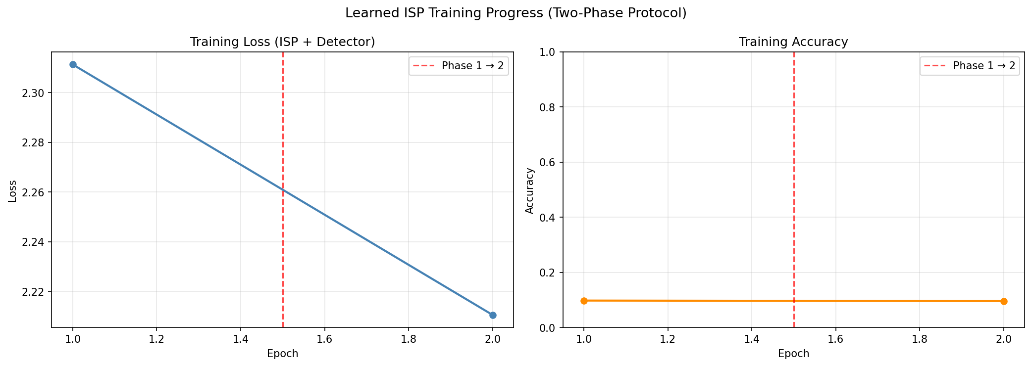
Left: loss decreasing over both phases. Right: accuracy improving. Red dashed line marks Phase 1 → Phase 2 transition.
Results¤
Before vs. After ISP Processing¤
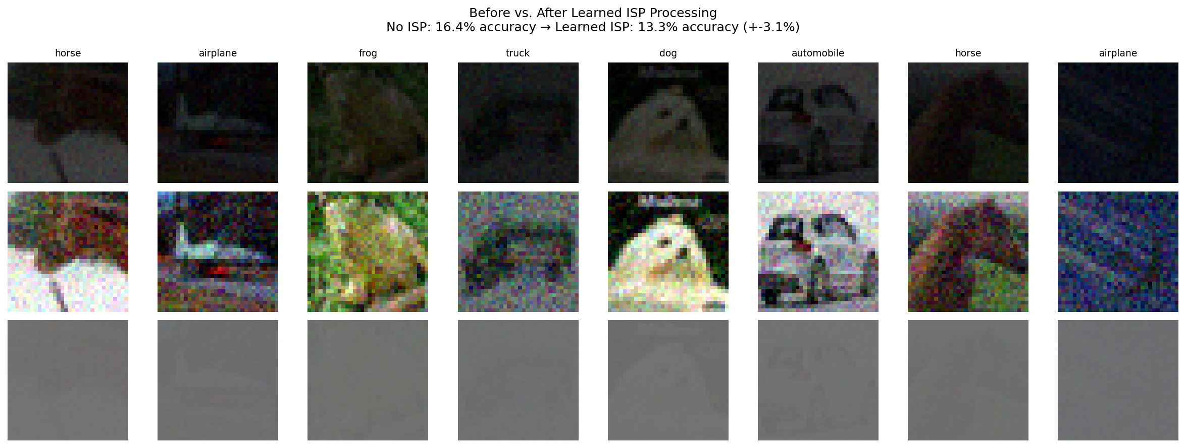
Top: raw dark images. Middle: dark images brightened 4x. Bottom: ISP-processed images — the learned pipeline enhances content for the classifier.
Learned ISP Parameters¤
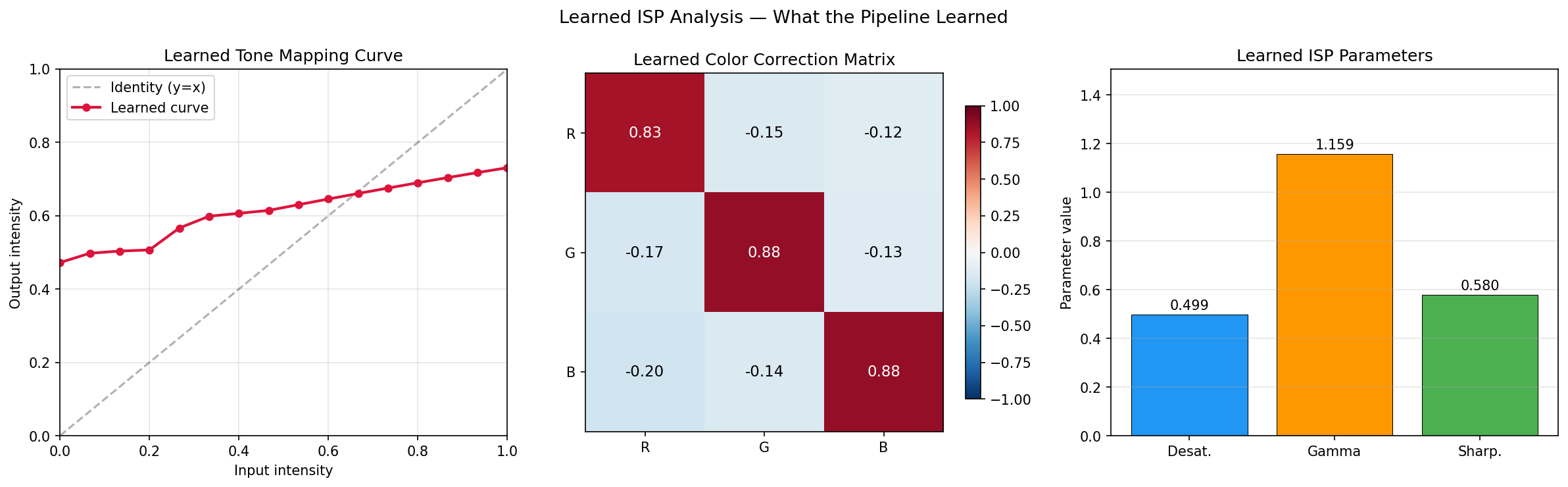
Left: learned tone mapping curve (vs. identity). Center: learned color correction matrix. Right: scalar ISP parameters.
Expected Results (Full Training on CIFAR-10)¤
| Configuration | Accuracy | Notes |
|---|---|---|
| No ISP (raw dark images) | ~10-15% | Near random (images too dark) |
| Fixed ISP (gamma=0.5) | ~40-50% | Standard brightening helps |
| Learned ISP | ~55-70% | Gradient-optimized for detector |
| AdaptiveISP (paper, RL) | ~30.2 mAP | Different dataset/metric (LOD) |
Key Takeaways¤
- Composition makes it natural:
CompositeOperatorModule(SEQUENTIAL)composes ISP stages into a differentiable pipeline. No manual loop or gradient wiring needed. - Gradient-based > RL: Direct gradient optimization is simpler and often more effective than RL-based ISP module selection.
- 37 parameters, big impact: The ISP pipeline has only 37 learnable parameters but dramatically changes what the detector "sees."
- Task-optimized processing: The learned ISP brightens dark images and enhances contrast — not for human viewing, but for detector accuracy.
Next Steps¤
- DADA Learned Augmentation — Operator library showcase
- DDSP Audio Synthesis — Extensibility to audio domain
Reference¤
- Wang et al., "AdaptiveISP: Learning an Adaptive ISP for Object Detection" (NeurIPS 2024) — arXiv:2410.22939
- OpenImagingLab/AdaptiveISP — Reference implementation