Distributed Data Loading with Sharding Guide

Metadata	Value
Level	Advanced
Runtime	~45 min
Prerequisites	Sharding Quick Reference, JAX device placement
Format	Python + Jupyter
Memory	~2 GB RAM per device

Overview

This in-depth guide covers distributed data loading patterns for multi-device JAX setups. You'll learn to shard data across GPUs/TPUs, optimize throughput for distributed training, and handle common pitfalls.

What You'll Learn

1. Design data parallelism strategies for different device topologies
2. Implement efficient sharded batch distribution
3. Profile and optimize distributed data loading
4. Handle edge cases (uneven batches, device failures)
5. Integrate sharded pipelines with distributed training

Coming from PyTorch?

PyTorch	Datarax
DistributedDataParallel(model)	Model with Mesh context
DistributedSampler	Data sharded via PartitionSpec
torch.distributed.all_reduce()	JAX handles via GSPMD
world_size, rank	mesh.axis_size, device position

Key difference: JAX's GSPMD provides automatic communication insertion based on sharding annotations.

Coming from TensorFlow?

TensorFlow	Datarax
tf.distribute.MirroredStrategy	Mesh with data axis
experimental_distribute_dataset	jax.device_put with sharding
strategy.scope()	with mesh: context
tf.distribute.Strategy.run()	jax.jit + sharding

Files

• Python Script: examples/advanced/distributed/02_sharding_guide.py
• Jupyter Notebook: examples/advanced/distributed/02_sharding_guide.ipynb

Quick Start

python examples/advanced/distributed/02_sharding_guide.py

Architecture

flowchart TB
    subgraph Source["Data Pipeline"]
        S[Source] --> P[Pipeline<br/>batch_size=128]
    end

    subgraph Mesh["1D Device Mesh (data axis)"]
        direction LR
        D0[GPU 0]
        D1[GPU 1]
    end

    P --> D0 & D1

Part 1: Understanding Data Parallelism

Sharding Dimensions

Dimension	Typical Sharding	Purpose
Batch	Sharded across devices	Data parallelism
Height/Width	Replicated	Full image on each device
Channels	Replicated	Full features on each device

Partition Specs

from jax.sharding import PartitionSpec as P

# Common partition specs
batch_sharded = P("data", None, None, None)  # (batch, H, W, C)
replicated = P(None, None, None, None)       # Full replication
model_sharded = P(None, None, None, "model") # Model parallelism

Part 2: Creating the Device Mesh

The guide builds a 1D mesh for pure data parallelism — all devices along a single "data" axis. This is what the script does:

import jax
import numpy as np
from jax.sharding import Mesh, NamedSharding, PartitionSpec

devices = jax.devices()
num_devices = len(devices)
use_sharding = num_devices >= 2

if use_sharding:
    # Create 1D mesh for pure data parallelism
    device_array = np.array(devices)
    mesh = Mesh(device_array, axis_names=("data",))
    print(f"Created mesh: {mesh.shape} with axis 'data'")
else:
    mesh = None
    print("Single device mode - will simulate sharding concepts")

Terminal Output:

Available devices: 2
Created mesh: (2,) with axis 'data'

Conceptual extension: 2D meshes

A 2D mesh combines data and model parallelism for large models. This guide does not use it — the snippet below is shown only to illustrate the pattern:

# Conceptual only — not exercised by this guide
if len(devices) >= 4:
    mesh_2d = Mesh(
        np.array(devices).reshape(2, 2),
        axis_names=("data", "model"),
    )

Part 3: Sharded Batch Distribution

A helper builds the right PartitionSpec for any array shape — sharding the first (batch) dimension across the "data" axis and replicating the rest:

def create_sharding_spec(shape, mesh, shard_first_dim=True):
    """Create appropriate PartitionSpec for a given shape."""
    if mesh is None:
        return None

    ndim = len(shape)
    if shard_first_dim and ndim > 0:
        # Shard first dim (batch), replicate rest
        spec = ("data",) + (None,) * (ndim - 1)
    else:
        # Fully replicate
        spec = (None,) * ndim

    return NamedSharding(mesh, PartitionSpec(*spec))

The pipeline itself is a standard Datarax pipeline with a preprocessing stage:

BATCH_SIZE = 128  # Total batch size across all devices
NUM_SAMPLES = 2048


def preprocess_image(element, key=None):
    """Standard image preprocessing."""
    del key
    image = element.data["image"].astype(jnp.float32) / 255.0
    return element.update_data({"image": image})


def create_pipeline(batch_size=BATCH_SIZE, num_samples=NUM_SAMPLES, seed=42):
    """Create CIFAR-10 data pipeline."""
    config = TFDSEagerConfig(
        name="cifar10",
        split=f"train[:{num_samples}]",
        shuffle=True,
        seed=seed,
        exclude_keys={"id"},
    )
    source = TFDSEagerSource(config, rngs=nnx.Rngs(seed))
    preprocessor = ElementOperator(
        ElementOperatorConfig(stochastic=False),
        fn=preprocess_image,
        rngs=nnx.Rngs(0),
    )
    return Pipeline(source=source, stages=[preprocessor], batch_size=batch_size, rngs=nnx.Rngs(0))

Each batch is distributed by applying the sharding to every array it contains:

def distribute_batch(batch, mesh, shard_batch_dim=True):
    """Distribute batch data across devices."""
    if mesh is None:
        return batch

    distributed = {}
    for key, array in batch.items():
        if hasattr(array, "shape"):
            sharding = create_sharding_spec(array.shape, mesh, shard_batch_dim)
            distributed[key] = jax.device_put(array, sharding)
        else:
            distributed[key] = array

    return distributed


# Distribute a batch within the mesh context
pipeline = create_pipeline()
test_batch = next(iter(pipeline))
with mesh:
    sharded_batch = distribute_batch(test_batch, mesh)
    print(f"  Image shape: {sharded_batch['image'].shape}")
    print(f"  Image sharding: {sharded_batch['image'].sharding.spec}")

Terminal Output:

Distributed batch:
  Image shape: (128, 32, 32, 3)
  Image sharding: PartitionSpec('data', None, None, None)

Part 4: Optimizing Throughput

The guide benchmarks throughput across a sweep of batch sizes. Each run warms up once, then times how quickly sharded batches become ready:

def benchmark_pipeline(batch_size, num_batches=20, mesh=None):
    """Benchmark pipeline throughput."""
    pipeline = create_pipeline(batch_size=batch_size, num_samples=batch_size * num_batches)

    # Warmup
    warmup_batch = next(iter(pipeline))
    if mesh is not None:
        with mesh:
            _ = distribute_batch(warmup_batch, mesh)

    # Benchmark
    pipeline = create_pipeline(batch_size=batch_size, num_samples=batch_size * num_batches)

    start = time.time()
    samples = 0

    if mesh is not None:
        with mesh:
            for batch in pipeline:
                sharded = distribute_batch(batch, mesh)
                _ = sharded["image"].block_until_ready()
                samples += batch["image"].shape[0]
    else:
        for batch in pipeline:
            _ = batch["image"].block_until_ready()
            samples += batch["image"].shape[0]

    elapsed = time.time() - start
    return samples / elapsed


# Sweep batch sizes
batch_sizes = [32, 64, 128, 256]
for bs in batch_sizes:
    tp = benchmark_pipeline(bs, mesh=mesh)
    print(f"  Batch size {bs}: {tp:.0f} samples/s")

Throughput rises with batch size as the fixed per-batch distribution overhead is amortized across more samples:

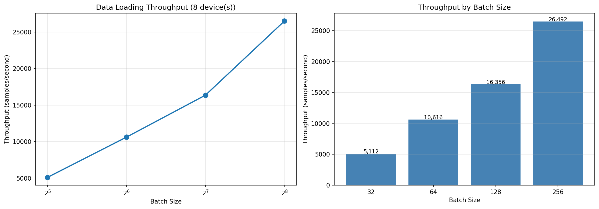
Data-loading throughput across batch sizes 32, 64, 128, and 256. Absolute numbers depend on your device count and hardware.

Part 5: Device Utilization

The guide also simulates device utilization during sharded data loading to illustrate how work spreads across devices:

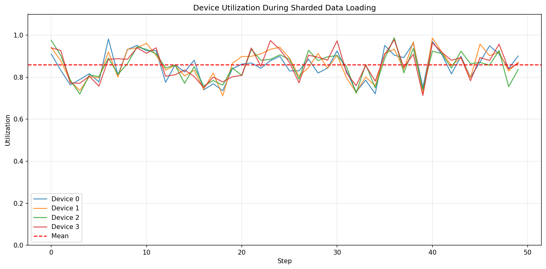
Simulated per-device utilization over the loading steps, with the mean marked.

Part 6: Batch Distribution

Finally, it visualizes how a single batch is split across devices:

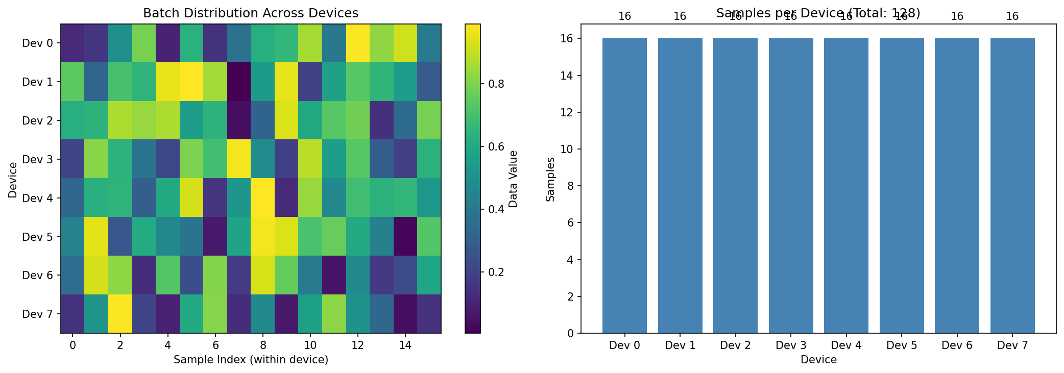
Left: batch samples distributed across devices. Right: samples per device for a total batch of 128.

Results Summary

Sharding Strategies

Strategy	Use Case	Mesh Shape
Pure Data Parallel	Most common	(N,) "data"
2D Data + Model	Large models	(D, M) "data", "model"
Pipeline Parallel	Very long sequences	(P,) "pipeline"

Performance Guidelines

Batch Size	Recommendation
< 32	Overhead may exceed benefit
64-256	Good balance
> 256	Check memory constraints

Key Takeaways

1. Batch size: Should be divisible by device count
2. Memory: Sharding reduces per-device memory linearly
3. Overhead: Distribution has fixed cost — larger batches amortize it
4. Mesh context: All sharded operations must be within mesh context
5. Fallback: Code should handle single-device gracefully

Next Steps

• Performance Guide - Further optimization
• Checkpointing - Distributed checkpoints
• End-to-End Training - Complete distributed training
• API Reference: Sharding - Complete API